Robust fitting and temporal smoothing

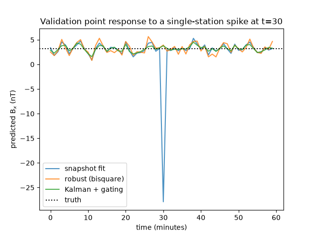
A large disturbance at a single station – a spike, a baseline jump, local interference – is inconsistent with any smooth ionospheric current system, but an ordinary least-squares fit will spread it across the entire interpolated map. This example compares three defenses:

1. the ordinary snapshot fit (contaminated),

2. robust IRLS weighting (fit(robust='bisquare')), which rejects the outlier spatially at each time step, and

3. pysecs.KalmanSECS with innovation gating, which couples the time steps and rejects observations inconsistent with the recent past.

import matplotlib.pyplot as plt
import numpy as np

from pysecs import SECS, KalmanSECS, T_df


R_E = 6378e3
rng = np.random.default_rng(11)

# A small grid of divergence-free SECs and a ground station network
lat_g, lon_g = np.meshgrid(np.linspace(-3, 3, 4), np.linspace(-3, 3, 4), indexing="ij")
sec_locs = np.column_stack([lat_g.ravel(), lon_g.ravel(), np.full(16, R_E + 110e3)])
nobs = 12
obs_locs = np.column_stack(
    [rng.uniform(-4, 4, nobs), rng.uniform(-4, 4, nobs), np.full(nobs, R_E)]
)

# Static true current system observed with noise for one hour at 1 min
true_amps = rng.normal(0, 1e4, 16)
B_true = np.tensordot(true_amps, T_df(obs_locs, sec_locs), (0, 2))
B_scale = np.max(np.abs(B_true))

ntimes = 60
times = np.arange(ntimes) * 60.0
noise = 0.05 * B_scale
B_obs = B_true[np.newaxis] + rng.normal(0, noise, (ntimes, nobs, 3))
obs_std = np.full_like(B_obs, noise)

# A 50x spike at station 0 halfway through the series
B_obs[30, 0, :] += 50 * B_scale

# Predict at a validation location far from the spiked station
pred_loc = np.array([[1.5, 1.5, R_E]])
B_val_true = np.tensordot(true_amps, T_df(pred_loc, sec_locs), (0, 2))[0]

# 1. Ordinary snapshot fit
snap = SECS(sec_df_loc=sec_locs)
snap.fit(obs_locs, B_obs, obs_std=obs_std, epsilon=1e-6)
pred_snap = snap.predict_B(pred_loc)

# 2. Robust IRLS fit
robust = SECS(sec_df_loc=sec_locs)
robust.fit(obs_locs, B_obs, obs_std=obs_std, epsilon=1e-6, robust="bisquare")
pred_robust = robust.predict_B(pred_loc)

# 3. Kalman smoother with innovation gating
kalman = KalmanSECS(SECS(sec_df_loc=sec_locs), tau=3600.0, gate_sigma=4.0)
kalman.fit(obs_locs, B_obs, times, obs_std=obs_std)
pred_kalman = kalman.predict_B(pred_loc)

fig, ax = plt.subplots()
minutes = times / 60
ax.plot(minutes, pred_snap[:, 0] * 1e9, label="snapshot fit", alpha=0.8)
ax.plot(minutes, pred_robust[:, 0] * 1e9, label="robust (bisquare)", alpha=0.8)
ax.plot(minutes, pred_kalman[:, 0] * 1e9, label="Kalman + gating", alpha=0.8)
ax.axhline(B_val_true[0] * 1e9, color="k", ls=":", label="truth")
ax.set_xlabel("time (minutes)")
ax.set_ylabel(r"predicted B$_x$ (nT)")
ax.set_title("Validation point response to a single-station spike at t=30")
ax.legend()
plt.show()