Internal / external field separation

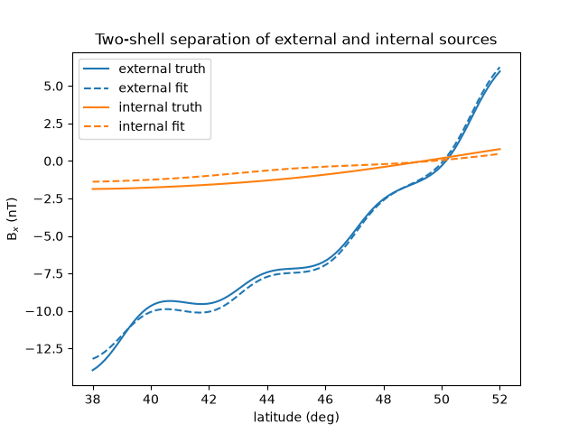
Ground magnetometers see both the ionospheric (external) currents and the telluric currents induced inside the Earth (internal). Placing divergence-free SECS on two shells – one in the ionosphere and one below the ground – separates the two contributions, as suggested in the conclusions of Amm and Viljanen (1999). All three magnetic field components are needed for the separation.

import matplotlib.pyplot as plt
import numpy as np

from pysecs import SECS, T_df


R_E = 6378e3
rng = np.random.default_rng(5)

# External shell in the ionosphere, internal image shell below ground
lat_g, lon_g = np.meshgrid(
    np.linspace(35, 55, 6), np.linspace(-10, 20, 8), indexing="ij"
)
ext_locs = np.column_stack(
    [lat_g.ravel(), lon_g.ravel(), np.full(lat_g.size, R_E + 110e3)]
)
int_locs = np.column_stack(
    [lat_g.ravel(), lon_g.ravel(), np.full(lat_g.size, R_E - 500e3)]
)

# Synthetic truth: internal currents mirror a fraction of the external
ext_amps = rng.normal(0, 1e4, ext_locs.shape[0])
int_amps = -0.35 * ext_amps

nobs = 30
obs_locs = np.column_stack(
    [rng.uniform(36, 54, nobs), rng.uniform(-9, 19, nobs), np.full(nobs, R_E)]
)
B_obs = np.tensordot(ext_amps, T_df(obs_locs, ext_locs), (0, 2)) + np.tensordot(
    int_amps, T_df(obs_locs, int_locs), (0, 2)
)
B_obs += rng.normal(0, 0.02 * np.max(np.abs(B_obs)), B_obs.shape)

# Fit both shells at once by stacking their SEC locations
both = SECS(sec_df_loc=np.vstack([ext_locs, int_locs]))
both.fit(obs_locs, B_obs, epsilon=0.01)

# Split the fitted amplitudes back onto individual shells for prediction
n_ext = len(ext_locs)
ext_fit = SECS(sec_df_loc=ext_locs)
ext_fit.sec_amps = both.sec_amps[:, :n_ext]
int_fit = SECS(sec_df_loc=int_locs)
int_fit.sec_amps = both.sec_amps[:, n_ext:]

# Compare along a latitude profile
profile = np.column_stack(
    [np.linspace(38, 52, 100), np.full(100, 5.0), np.full(100, R_E)]
)
B_ext_true = np.tensordot(ext_amps, T_df(profile, ext_locs), (0, 2))
B_int_true = np.tensordot(int_amps, T_df(profile, int_locs), (0, 2))

B_ext_pred = ext_fit.predict_B(profile)
B_int_pred = int_fit.predict_B(profile)

fig, ax = plt.subplots()
lats = profile[:, 0]
ax.plot(lats, B_ext_true[:, 0] * 1e9, "C0", label="external truth")
ax.plot(lats, B_ext_pred[:, 0] * 1e9, "C0--", label="external fit")
ax.plot(lats, B_int_true[:, 0] * 1e9, "C1", label="internal truth")
ax.plot(lats, B_int_pred[:, 0] * 1e9, "C1--", label="internal fit")
ax.set_xlabel("latitude (deg)")
ax.set_ylabel(r"B$_x$ (nT)")
ax.set_title("Two-shell separation of external and internal sources")
ax.legend()
plt.show()