Automatic SECS grid generation

Choosing a SECS grid by hand means picking a spacing, a padding margin around the stations, and checking that no pole lands on top of a station. pysecs.SECS.from_observations() (built on pysecs.make_grid()) automates this from the observation network alone: the spacing defaults to the median nearest-neighbor station separation and the grid is padded several cells beyond the station footprint so that currents just outside the network do not alias onto the grid edges.

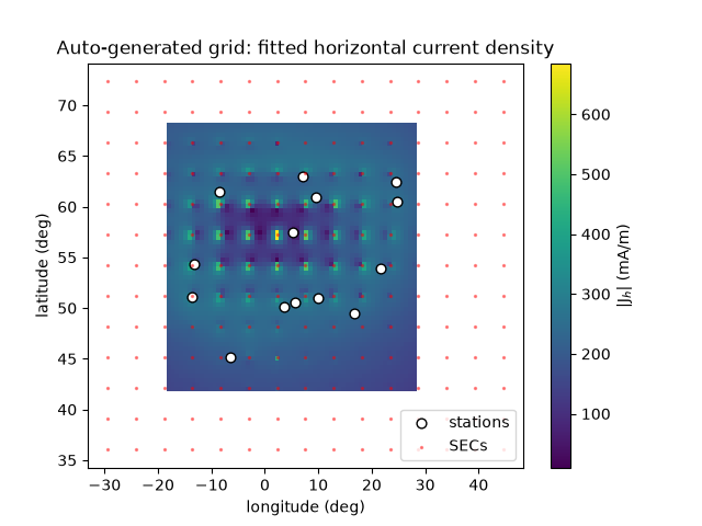
auto-generated grid: 195 SECs

import matplotlib.pyplot as plt
import numpy as np

from pysecs import SECS, T_df, make_grid


R_E = 6378e3
R_I = R_E + 110e3
rng = np.random.default_rng(7)

# An irregular ground station network, as one would get from a real
# observatory list rather than a hand-picked regular layout
nobs = 14
obs_lat = rng.uniform(45, 65, nobs)
obs_lon = rng.uniform(-15, 25, nobs)
obs_loc = np.column_stack([obs_lat, obs_lon, np.full(nobs, R_E)])

# A synthetic "true" current system on a fine grid, used to generate
# synthetic station observations
truth_grid = make_grid(obs_loc, R_I, spacing=1.0)
truth_amps = (
    1e4
    * np.exp(-(((truth_grid[:, 0] - 57) / 6) ** 2))
    * np.cos(np.deg2rad(truth_grid[:, 1]) * 3)
)
B_obs = np.tensordot(truth_amps, T_df(obs_loc, truth_grid), (0, 2))

# Automatically generate the fitting grid from the station locations
# alone -- no manually chosen spacing, bounds, or pole positions
secs = SECS.from_observations(obs_loc, r_shell=R_I)
secs.fit(obs_loc, B_obs)
print(f"auto-generated grid: {secs.nsec} SECs")

# Predict the current density on a map for plotting
plat, plon = np.meshgrid(
    np.linspace(42, 68, 60), np.linspace(-18, 28, 60), indexing="ij"
)
pred_loc = np.column_stack([plat.ravel(), plon.ravel(), np.full(plat.size, R_I)])
J_pred = secs.predict_J(pred_loc)
J_mag = np.linalg.norm(J_pred[:, :2], axis=-1).reshape(plat.shape)

fig, ax = plt.subplots()
pcm = ax.pcolormesh(plon, plat, J_mag * 1e3, shading="auto", cmap="viridis")
ax.scatter(obs_lon, obs_lat, c="w", edgecolor="k", s=40, label="stations")
ax.scatter(
    secs.sec_df_loc[:, 1], secs.sec_df_loc[:, 0], c="r", s=2, alpha=0.4, label="SECs"
)
ax.set_xlabel("longitude (deg)")
ax.set_ylabel("latitude (deg)")
ax.set_title("Auto-generated grid: fitted horizontal current density")
ax.legend(loc="lower right")
fig.colorbar(pcm, ax=ax, label=r"|J$_h$| (mA/m)")
plt.show()