Curl free magnetic field

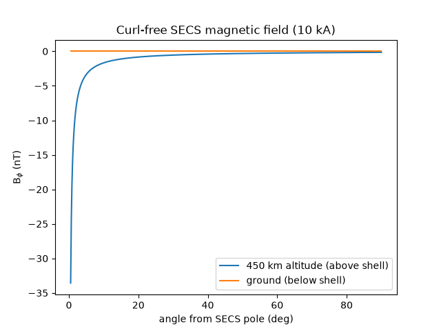
The magnetic field of a curl-free SECS (with its associated radial field-aligned currents) is identically zero at and below the current shell – Fukushima’s theorem – which is why ground magnetometers can never constrain curl-free amplitudes. Above the shell the field is purely azimuthal (Vanhamäki and Juusola 2020, Equation 2.15). This example shows the angular profile at satellite altitude and on the ground.

import matplotlib.pyplot as plt
import numpy as np

from pysecs import SECS


# Radius of Earth
R_E = 6378e3
# Current shell at 100 km altitude
R_I = R_E + 100e3

# Pole of the current system at the North Pole
sec_loc = np.array([90.0, 0.0, R_I])

system_cf = SECS(sec_cf_loc=sec_loc)

# Fit unit currents since we aren't fitting to any data,
# then scale to a 10 kA system
system_cf.fit_unit_currents()
I0 = 10000

# Observation points along a meridian, from the pole to the equator
angles = np.linspace(0.5, 90, 500)
lats = 90 - angles

# On the ground (below the shell) and at 450 km altitude (above it)
obs_ground = np.column_stack([lats, np.zeros_like(lats), np.full_like(lats, R_E)])
obs_sat = np.column_stack([lats, np.zeros_like(lats), np.full_like(lats, R_E + 450e3)])

B_ground = I0 * system_cf.predict_B(obs_ground)
B_sat = I0 * system_cf.predict_B(obs_sat)

fig, ax = plt.subplots()
# The azimuthal (eastward) component carries the entire field
ax.plot(angles, B_sat[:, 1] * 1e9, label="450 km altitude (above shell)")
ax.plot(angles, B_ground[:, 1] * 1e9, label="ground (below shell)")
ax.set_xlabel("angle from SECS pole (deg)")
ax.set_ylabel(r"B$_\phi$ (nT)")
ax.set_title("Curl-free SECS magnetic field (10 kA)")
ax.legend()
plt.show()